From Past to Present - An Analytical Overview of Singapore’s Parliamentary Elections
Background
At the People’s Action Party (PAP) conference on November 24, 2024, Prime Minister Lawrence Wong highlighted the political challenges Singapore is currently facing. Unlike in the past, he emphasised that the PAP can no longer assume there are “safe seats” in the General Election (GE) or that the party will automatically secure a stable government No chance of ‘opposition wipe-out’ in next GE: PM Lawrence Wong,”.
In this assignment, you will compose a report to analyse and document the history and recent developments of parliamentary elections in Singapore from a data analyst’s perspective. The objective is to present an objective, data factual, and comprehensive overview of Singapore’s parliamentary elections since their inception in 1955 leading up to GE 2025. Your primary data source will be from Data.gov.sg. Except for electoral boundaries, where geojson data are provided separately, all data must be extracted via the data.gov.sg’s API.
Executive Summary
The 2025 parliamentary election signifies an important milestone as Singapore welcomes its 60th year of independence. In preparation for the upcoming election, this report aims to provide a comprehensive analysis on Singapore’s electoral history, modifications to the electoral system via the introduction of Group Representation Constituencies (GRC) scheme in 1988, followed by an in-depth analysis to performances of political parties as well as recent developments to the electoral landscape.
The analysis portrays the dominance of the People’s Action Party (PAP) in votes and seats post-independence. Despite the rise of opposition parties, PAP maintained its position as the ruling party. Additionally, the intent of introducing GRC scheme was to ensure a multiracial parliament. However, it also gave PAP an advantage as opposition parties struggle to compete initially due to limited resources.
While PAP continues to assert its dominance in the elections as the ruling party, they should aim to regain trust from residents residing in East and West Coast GRCs as winning margins were slim. On the other hand, WP has expanded their influence in parliament through capturing Aljunied and Sengkang GRCs in recent times. However, more work has to be done to defend Sengkang GRC due to slim winning margins and resignation of a member in light of a scandal.
Regardless on parties’ strategy and ethos, the utmost agenda for the 2025 parliamentary election shall be filling up all vacated seats to allow a holistic representation of Singapore’s voice in parliament.
1.0 Introduction to Singapore’s General Election
As Singapore marks her 60th year of independence, another significant event is unfolding behind the scenes – The 2025 Parliamentary Elections. Singapore’s electoral footprints can be traced back to 1955, where she held her first Legislative Assembly elections. It was deemed a landmark election as legislators were elected through popular ballot rather than appointment by British colonial authorities. Since then, Singapore has re-elected her legislators through the electoral system on a first-past-the-post basis whereby the candidate(s) with the greatest number of votes win the constituency, regardless of the winning margin.
Under the electoral system, there are three categories of members that form the Parliamentary House (i.e. Members of Parliament (MP)). The first category consists of members who are directly elected by their constituencies, coming from either the Single Member Constituency (SMC) or a Group Representation Constituency (GRC) that they contest in. The second category comprises the Non-Constituency Members (NCMP) and the final category of members being the Nominated Member of Parliament (NMP). At present, there are a total of 96 MPs, of which 87 are elected by Singaporeans, 2 from NCMP and 7 from NMPs. The size of a constituency is determined by electoral boundaries committee where parameters of an existing constitution may be redrawn before each parliamentary election.
The Parliamentary Elections encompass both the General Elections (GE) and by-elections with a maximum serving term of five years. However, it may be dissolved before the expiry of its five-year term subject to the President’s approval. The GE must be held within three months of dissolving the Parliament whereas by-elections are held when a seat for SMC or instances where all MPs for a GRC vacate their seats.
In preparation for Singapore’s upcoming elections in forming the 15th Parliament, this report aims to present a comprehensive analysis to Singapore’s electoral results, performances of political parties, as well as an in-depth analysis on recent developments to Singapore’s electoral landscape to inform readers who are participating in the voting process.
2.0 Overview Analysis of Parliamentary Elections
Among 39 political parties, the People’s Action Party (PAP) and Workers’ Party (WP) have participated in most, if not all parliamentary elections. Therefore, a new classification has been created to group other opposition parties and independent candidates as “Other Opposition” for ease of analysis where applicable.
2.1 Number of Political Parties Over Time
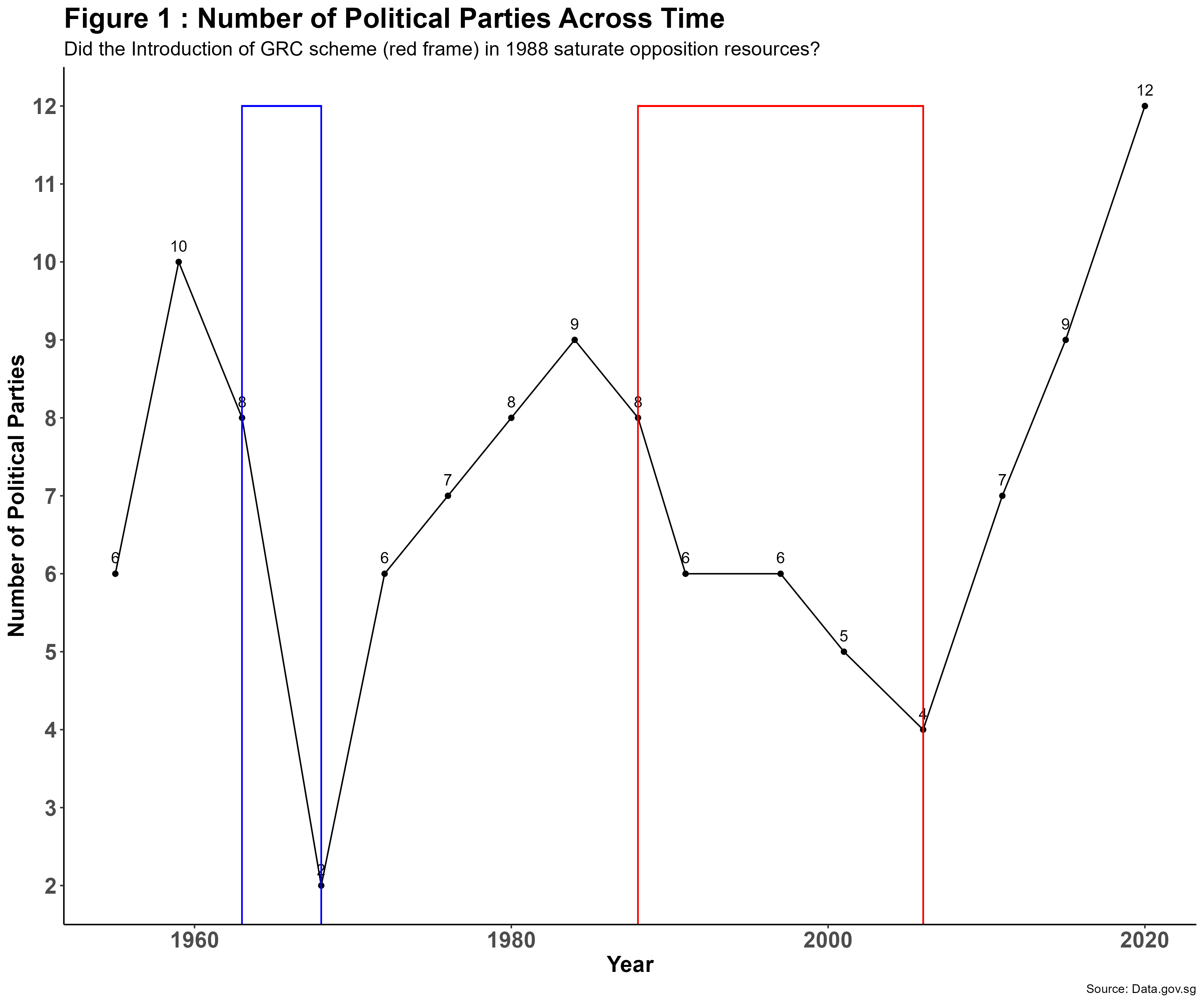
From Figure 1, the number of political parties in Singapore significantly plunged between the 1963 and 1968 (8 parties vs 2 parties) denoted within the blue frame. This sharp reduction in parties and intensity of competition came after Singapore’s separation from the Federation of Malaysia in 9 August 1965 where several opposition parties boycotted the elections and withdrew from contesting. Following the unrest, Singapore had gradually regained political stability, leading to a healthy contest for seats depicted by an increase in political parties entering the contest. Between 1968 and 1988, the number of political parties expanded from 2 to 8 parties.
However, a second reduction to the number of parties were noted within the red frame between 1988 to 2006. During this period, the significant electoral change made was the introduction of the Group Representation Constituencies (GRC) scheme. The intent was for contesting parties to fill at least 1 candidate from a minority racial community (e.g. Malay, Indians, Eurasians), ensuring a multiracial parliament. Subsequent to 2006 parliamentary elections, the number of political parties rose from 4 parties to 12 parties, which coincided with the rise of social media and digital marking platforms.
2.2 Analysis by Votes
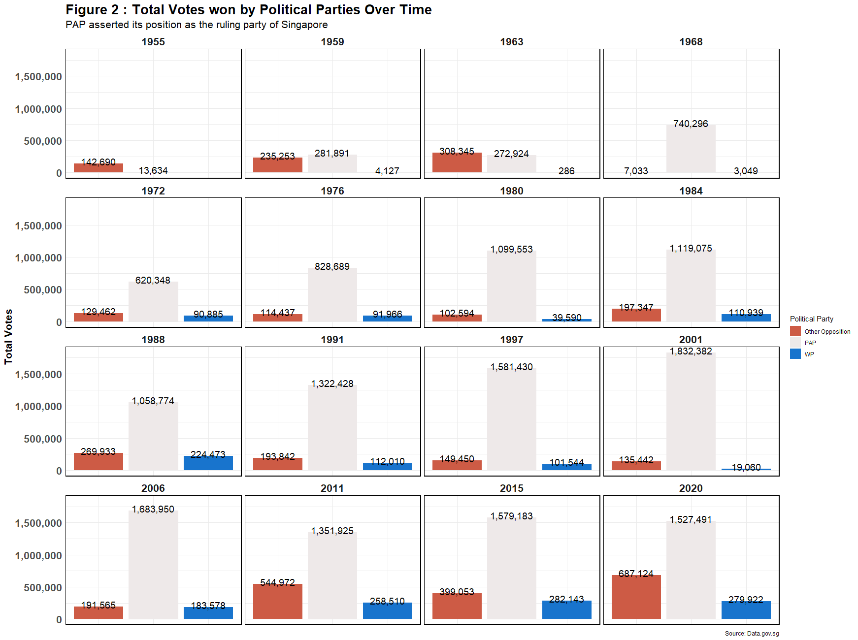
Barring the earlier elections held before Singapore’s independence in Figure 2, it is evident that PAP has gathered the most votes throughout the elections. In addition, PAP manages to hold its weight as the number of opposition parties grew, even as many as 9 during the 1984 parliamentary election. At its peak, PAP also received 1.83 Million votes from the 2001 parliamentary elections. However, the number of votes gathered by the PAP in recent parliamentary elections have plateaued between 2006 and 2020, which may be attributable by the boom in number of opposition parties and increased presence due to the rise of social media and digital marketing.
On the other hand, WP and other opposition parties experienced a series of ebb and flow in votes received throughout the parliamentary elections. The former achieved their first breakthrough between 1972 and 1988 and recent breakthroughs between 2006 and 2020 while the latter experienced a heavy decline in 1968 due to political boycotts before restoring some footing in recent times. Both parties also experienced a decline in votes received between 1988 and 2001, which coincided with the introduction of GRC scheme in 1988 (refer to section 2.4).
Despite the rise of opposition parties and plateauing of votes received in recent times, PAP asserted its position as the ruling party of Singapore. Next, we shall also analyse average votes received from every parliamentary elections in percentage form using a line chart.
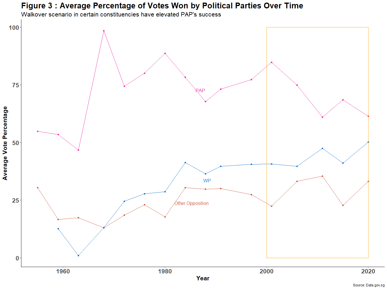
Analysing votes depicted from another perspective (Figure 3) using a line chart, PAP has been popular across time given the huge gap relative to opposition parties. At its peak, PAP amassed an average vote percentage of 98.2%. This phenomenon can be explained by the presence of a “walkover” scenario where no other party contested for a certain constituency. Therefore, walkovers have artificially elevated PAP’s success in earlier years. Additionally, the initial political instability post-independence also contributed to the increase in walkover scenarios.
Following stabilisation of Singapore’s political scene, coupled with the rise in number of parties contesting, popularity votes had been transferred from PAP to WP and other opposition parties who offers fresh perspective and ideology between 1963 and 1988. However, PAP has regained a considerable amount of popularity from voters due to the introduction of GRC scheme. Under the GRC scheme, political parties are expected to fill multiple candidates with at least 1 member coming from a minority racial community. This change initially saturated resources for both WP and other opposition parties due to the vast differences in network and recruiting strength relative to PAP (refer to Section 2.4).
As WP and other opposition parties adapted to the changes in system, coupled with the rise of social media and digital marketing, their popularity resurged as they became more active in contesting for GRC constituencies (yellow frame). PAP also regained some popular vote in the 2015 parliamentary elections as Singapore celebrated its 50th year of independence, which has been the focal point of PAP’s election strategy.
Therefore, the popularity of a party can be influenced by external factors such as changes made to electoral system, campaigning strategies, quality of competition and the presence of walkover scenarios.
2.3 Analysis by Seats Won
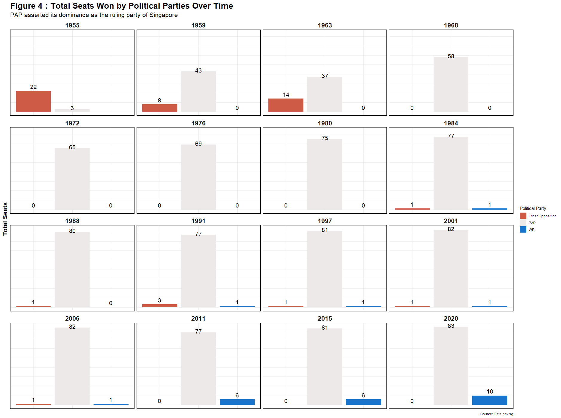
From Figure 4, PAP has been influential in forming Singapore’s parliament post-independence. Between 1968 and 1980, PAP even won all seats that were eligible for contest. However, their monopoly streak ended in 1984, where the Singapore Democratic Party (SDP) took the seat in Potong Pasir SMC, with WP securing Anson SMC. PAP eventually recaptured Potong Pasir in 2011. Although WP lost Anson in 1988, they went on to win Hougang SMC in 1991 and has firmly anchored this seat for 3 decades. The 2011 election was also a historic moment for WP as seats were secured for Aljunied GRC, the first opposition to do so. WP held on to Aljunied GRC in subsequent elections. In 2020, WP achieved another historic milestone as they secured seats for Sengkang GRC.
In essence, it is conclusive that opposition parties, especially WP, are gaining recognition and trust from Singaporeans over time. It is further complemented by the rising amount of votes won. Nonetheless, a deeper dive into the results by respective schemes shall be conducted to better analyse how votes have been distributed at the constituency level and draw additional insights.
2.4 Introduction and Analysis of GRC Scheme
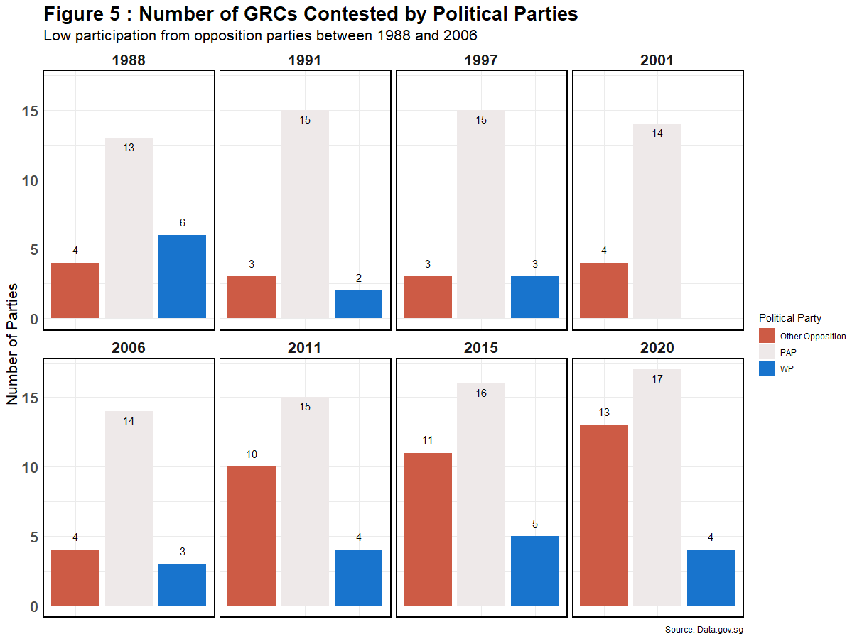
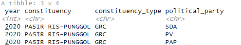
Through Figure 5, opposition’s involvement in contesting for GRC remained low between 1988 and 2006. Analysing in tandem with the declining number of oppositions present within the same period (Figure 1 red frame), it becomes apparent that opposition resources did saturate following the introduction of GRC scheme. Nonetheless, opposition parties managed to gain traction and begun pulling their weight between 2011 and 2020 as they established their identity and footing in Singapore’s political scene. For instance, there were 2 oppositions that contested for Pasir Ris-Punggol GRC alongside PAP.
The rise of social media and digital marketing also boosted oppositions push in gaining recognition. However, vast differences in resources and reputation were still prominent as Walkover scenario was present as recent as 2011 parliamentary election, further highlighting the limited/stretched resources on opposition parties while PAP consistently contests for all GRC seats.
2.5 Analysis of SMC Results
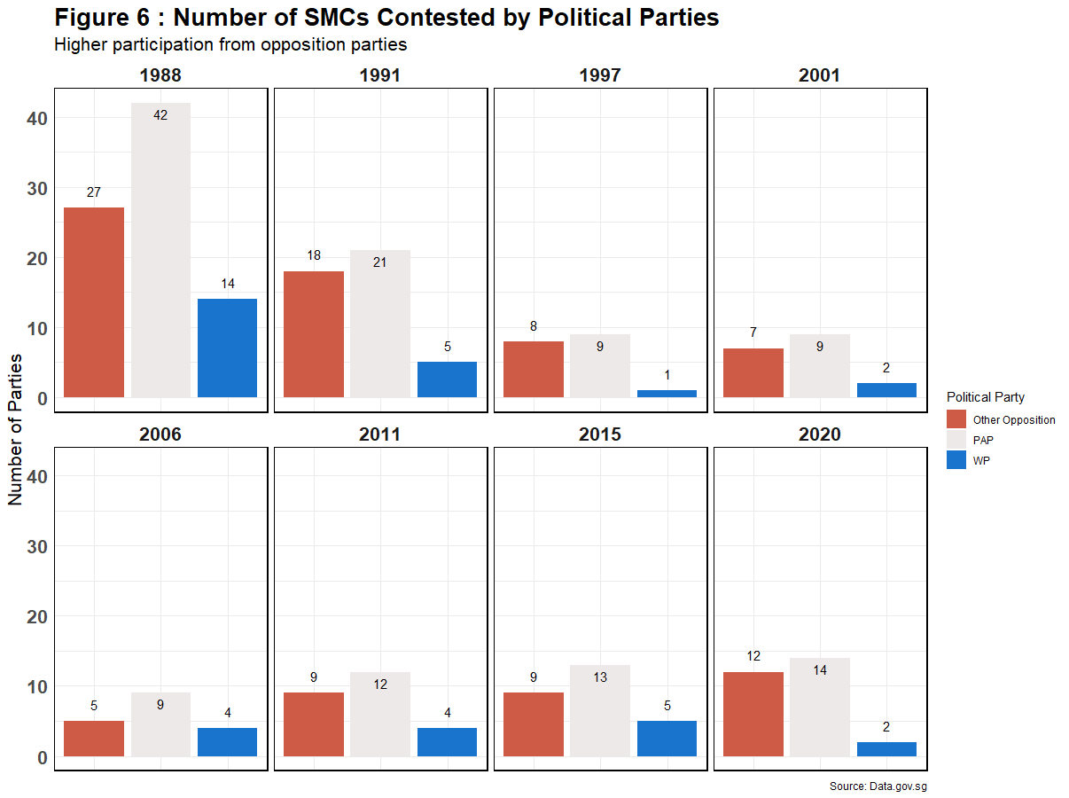
Figure 6 paints an opposite narrative from Figure 5. Opposition parties remained highly involved in their contest for SMCs as most constituencies were represented by at least 1 opposition candidate. In addition, the last time a walkover scenario happened was dated further back in 1991 relative to GRC’s last walkover scenario in 2011.
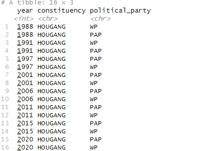
Another interesting observation was that no SMCs had more than 2 opposition parties contesting for the same constituency since 1988. Therefore, opposition parties may have coordinated among themselves on a specific constituency they want to contest in as a solution to distribute limited resources. For instance, no opposition party other than WP contested for Hougang SMC since 1988 as it is publicly referred to as WP’s “stronghold” ward.
In essence, evidence suggests that the introduction of GRC scheme has given PAP the advantage in forming parliament quickly given their vast resources and connections, allowing them to fill seats in an efficient manner.
2.6 Flipping of Seats from By-Elections
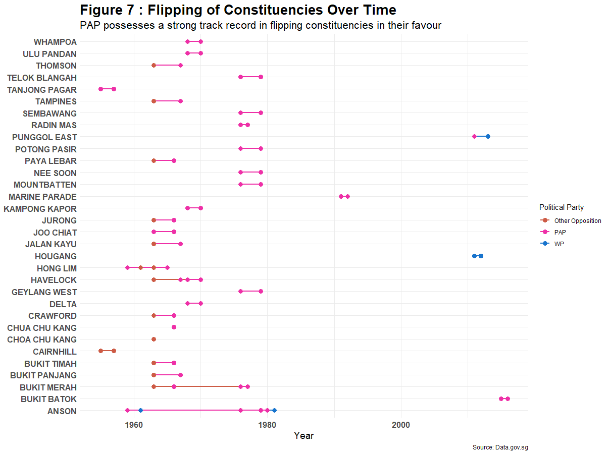
Throughout the history of Singapore’s by-election results shown in Figure 7, the PAP possessed a tremendous record in flipping and defending its seat in parliament for most constituencies. Before 1988, Anson was also the most flipped constituency, often changing seats between PAP and WP before being absorbed into Tiong Bahru GRC in 1988, which was won by PAP. Post split of GRC/SMC scheme, WP should be credited for their performances in by-elections as they managed to flip Punggol East SMC, which was later absorbed under Sengkang GRC in 2020 where WP won as well as Hougang SMC, where WP defended their seat.
2.7 Analysis of Recent Political Landscape and Recent Developments
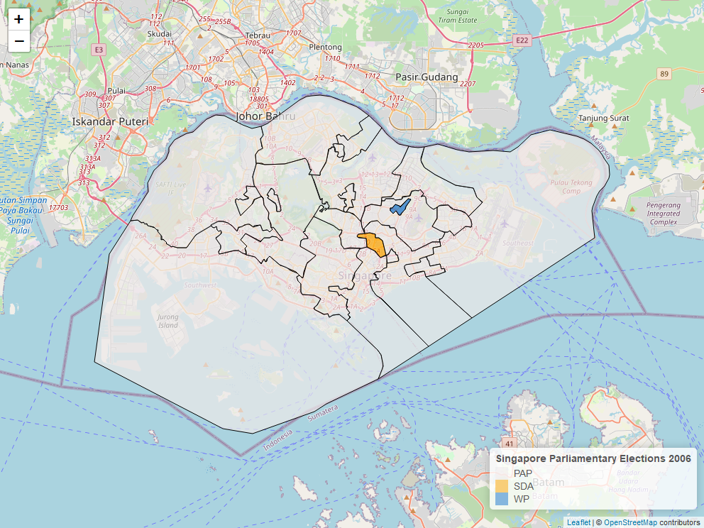
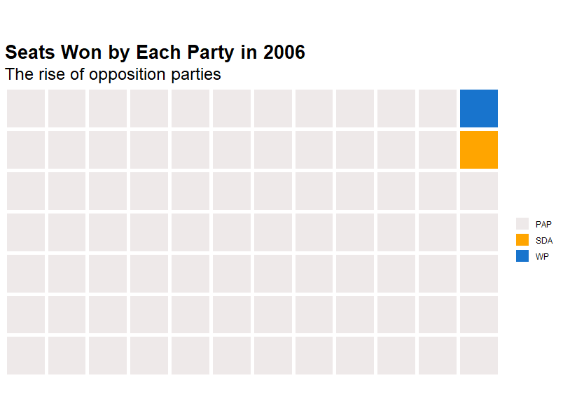
2.7.1 Results of 2006 Parliamentary Election:
Looking at charts depicting 2006 parliament election above, the only 2 SMCs that PAP did not capture were Potong Pasir and Hougang SMCs, while securing a whopping 82 of 84 seats.
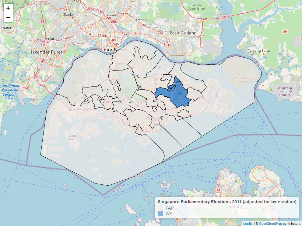
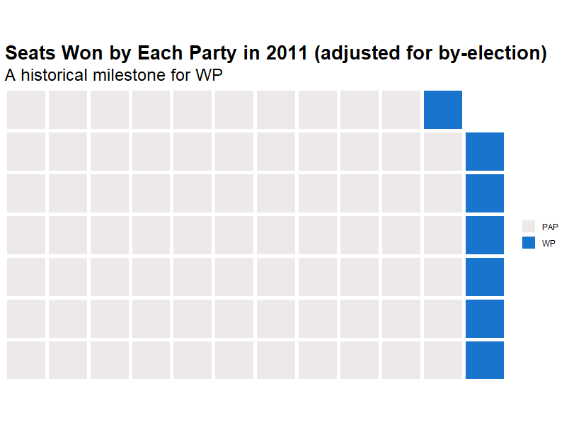
2.7.2 Results of 2011 Parliamentary Election (adjusted for by-election):
The 2011 parliamentary election was earmarked as a historical milestone for WP as they became the first opposition to capture a GRC (Aljunied GRC). Additionally, WP also defended Hougang SMC in the 2012 by-election while flipping Punggol East SMC in the 2013 by-election following expulsion of incumbent MPs for both SMCs. This took WP’s total seats in parliament from 1 seat in 2006 to 7 seats in 2013.
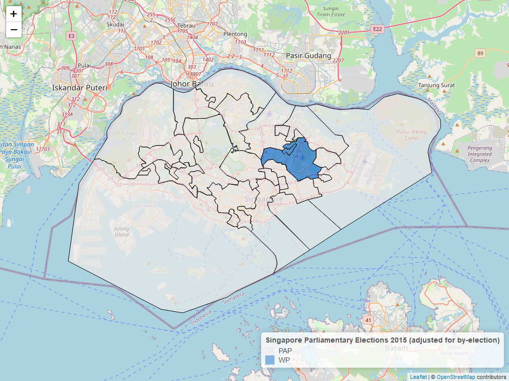
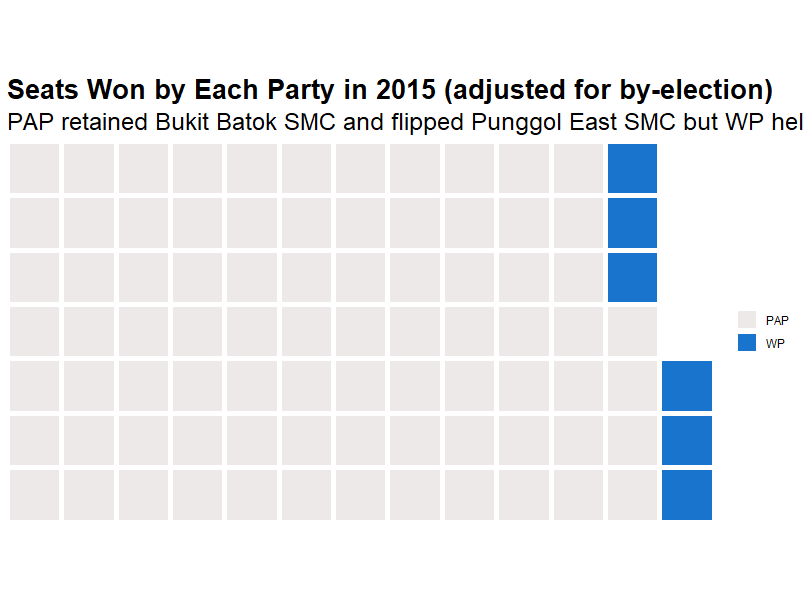
2.7.3 Results of 2015 Parliamentary Election (adjusted for by-election):
The 2015 parliamentary election was almost a status quo following 2013 by-election in terms of seats won except for Punggol East SMC, where PAP manages to recapture the seat from WP. The only by-election occurred in 2016 for Bukit Batok SMC due to the sudden resignation of incumbent MP where PAP defended their seat. Therefore, seat composition in parliament remained unchanged post 2016 by-election.
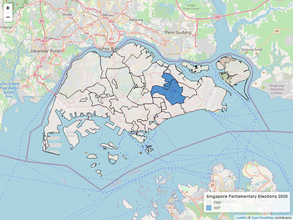
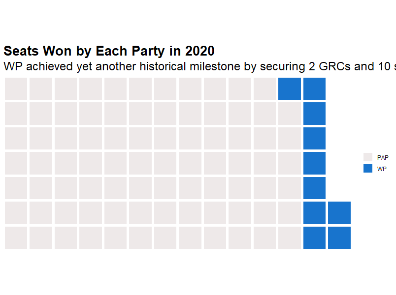
2.7.4 Results of 2020 Parliamentary Election:
The 2020 parliamentary elections marked another significant milestone for WP as they captured their second GRC (Sengkang GRC) while defending both Hougang SMC and Aljunied GRC, bringing their total seat in parliament to 10 seats.
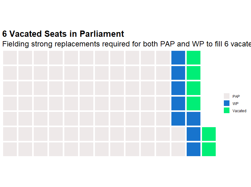
2.7.5 Vacating Parliamentary Seats
ecently, Singapore’s political landscape have been heavily impacted by scandals and negative limelight, leading to the highest number of resignations by MPs since the political boycott in 1968. WP vacated 2 seats and the PAP vacated 4 seats ahead of the 2025 parliamentary election. Adjustments were made to deduct vacated seats from each party before visualising them via a waffle plot.
3.0 Conclusion
To conclude, the utmost priority for the 2025 parliamentary election will be to fill all vacated seats so that Singaporean’s voices are effectively advocated for in parliament. With recent negative events affecting reputations of both PAP and WP, trust would have to be reestablished with Singaporeans. All arguments considered, PAP is expected to be given the mandate and form the 15th Singapore Parliament given their impressive governing record and dominance in elections. However, PAP is unlikely to regain control over Aljunied GRC due to the presence of a formidable team as well as Hougang SMC, where the seat has been firmly held by WP for three decades, anchoring itself as a stronghold constituency.
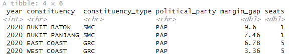
PAP’s extent of control in parliament is contingent on favorable swing on Sengkang GRC, and whether trust could be regained from voters in constituencies where PAP’s winning margins have been slim depicted below. In particular, both East and West Coast GRCs are PAP’s worst performing constituencies/GRCs from 2020. Therefore, it is paramount for PAP to retain them as 10 seats will be lost in the event of a flip.
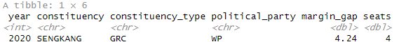
Although WP has achieved their medium-term ethos of representing Singaporeans voice in parliament, the next phase of WP’s development should be to extend their influence through fielding strong candidates to both East and West Coast GRCs in an attempt to secure additional seats. Concurrently, WP should also focus on fielding a strong replacement in defending their seat for Sengkang GRC given the slim winning margin and resignation of an elected member due to a scandal.
For other opposition parties, their focus should be on enhancing party’s image through expansion of outreach programmes to gain recognition and buy in towards their party’s ethos from Singaporeans.
Till this end, I strongly believe that the upcoming election will be about a battle of fine margins for our voices to be heard in parliament. See you at the polls!
4.0 Data Extraction via an API
Data is extracted from https://data.gov.sg/ through an Application Programming Interface (API) with the Elections Department as the referenced agency using ‘get()’ and ‘fromJSON()’ functions reproduced below for reference:
1
2
3
4
5
6
7
8
9
10
11
12
13
14
15
16
17
18
19
20
21
22
23
24
25
26
27
28
29
30
31
32
33
34
35
36
37
38
39
40
41
42
43
44
45
46
47
48
49
50
51
52
53
54
55
56
57
58
## For extracting external data through an GET API call from data.gov.sg
library(httr) # To use get() to extract data from data.gov.sg into JSON format
library(jsonlite) # To use fromJSON() to extract JSON content into a data frame

## 1) List of Political Parties

# URL to extract the data from data.gov.sg
url.pp <- GET("https://data.gov.sg/api/action/datastore_search?resource_id=d_ef163fd9ebc3c2f21032c29da3bd3f77&limit=3000")

# Extract content from raw JSON file
raw.pp <- fromJSON(rawToChar(url.pp$content), flatten = T)

# Extracting the data frame and saving into RMD
df.pp <- raw.pp$result$records

## 2) Parliamentary Election - Registered Electors, Rejected Votes and Spoilt Ballots

# URL to extract the data from data.gov.sg
url.re <- GET("https://data.gov.sg/api/action/datastore_search?resource_id=d_fdfb854fcb7428b29734d2e0c0674220&limit=3000")

# Extract content from raw JSON file
raw.re <- fromJSON(rawToChar(url.re$content), flatten = T)

# Extracting the data frame and saving into RMD
df.re <- raw.re$result$records

## 3) Parliamentary General Election Results by Candidate

# URL to extract the data from data.gov.sg
url.ge.results <- GET("https://data.gov.sg/api/action/datastore_search?resource_id=d_581a30bee57fa7d8383d6bc94739ad00&limit=3000")

# Extract content from raw JSON file
raw.ge.results <- fromJSON(rawToChar(url.ge.results$content), flatten = T)

# Extracting the data frame and saving into RMD
df.ge.results <- raw.ge.results$result$records

## 4) Parliamentary By-Election - Registered Electors, Rejected Votes and Spoilt Ballots

# URL to extract the data from data.gov.sg
url.re.by.election <- GET("https://data.gov.sg/api/action/datastore_search?resource_id=d_f237c2349833df4247d2f93102e714d5&limit=3000")

# Extract content from raw JSON file
raw.re.by.election <- fromJSON(rawToChar(url.re.by.election$content), flatten = T)

# Extracting the data frame and saving into RMD
df.re.by.election <- raw.re.by.election$result$records

## 5) Parliamentary By-Election Results by Candidate

# URL to extract the data from data.gov.sg
url.be.results <- GET("https://data.gov.sg/api/action/datastore_search?resource_id=d_ba8da764a37ca36b34e4e5ad866294f8&limit=3000")

# Extract content from raw JSON file
raw.be.results <- fromJSON(rawToChar(url.be.results$content), flatten = T)

# Extracting the data frame and saving into RMD
df.be.results <- raw.be.results$result$records
Electoral boundary data is extracted from the zip file provided. As the files are in GEOJSON format, the data source name function ‘dsn()’ is applied to specify the file, followed by ‘st_zm()’ to remove z-axis. The ‘read_sf()’ function is then used to convert into a simple feature data frame reproduced below for reference:
1
2
3
4
5
6
7
8
9
10
11
12
# Load 'sf' package
library(sf)

# Extract and convert boundaries data into sf data frames
df.boundaries.2006 <- read_sf(dsn = 'ElectoralBoundary2006GEOJSON.geojson')  %>%
  st_zm() # Strip away z-axis
df.boundaries.2011 <- read_sf(dsn = 'ElectoralBoundary2011GEOJSON.geojson')  %>%
  st_zm() # Strip away z-axis
df.boundaries.2015 <- read_sf(dsn = 'ElectoralBoundary2015GEOJSON.geojson')  %>%
  st_zm() # Strip away z-axis
df.boundaries.2020 <- read_sf(dsn = 'ElectoralBoundary2020GEOJSON.geojson')  %>%
  st_zm() # Strip away z-axis
4.1 Data Exploration
All imported data shall be explored using ‘glimpse()’ and ‘skim()’ functions to sieve out inconsistencies that requires further cleaning. The preliminary ‘glimpse()’ shows that the classes for numeric data are incorrect while the preliminary ‘skim()’ shows some missing observations in the data frames.
1
2
3
4
5
6
7
8
9
10
11
12
13
14
15
16
17
18
19
20
21
# Load 'tidyverse' package
library(tidyverse)

glimpse(df.pp)
glimpse(df.re)
glimpse(df.re.by.election)
glimpse(df.ge.results)
glimpse(df.be.results)
glimpse(df.boundaries.2006)
glimpse(df.boundaries.2011)
glimpse(df.boundaries.2015)
glimpse(df.boundaries.2020)

# Load 'skimr' package
library(skimr)

skim(df.pp)
skim(df.re)
skim(df.re.by.election)
skim(df.ge.results)
skim(df.be.results)
4.2 Data Pre-processing
From the data exploration process, several inconsistencies were noted:
- Most columns were presented in character class;
- Inconsistent naming of political party across data frames;
- ‘year’ variable is presented as a character class;
- “NA” is present in ‘df.re’, ‘df.re.by.election’, ‘df.ge.results’ and ‘df.be.results’ data frames;
- The ‘description’ variable within geoJSON boundaries files contains the constituency names. However, it is difficult to read/deduce at first glance.
Following are the data pre-processing steps performed (refer to “5.0 Data Appendix” for detailed discussion):
- Remove ‘_’ within ‘_id’ variable;
- Rename ‘party’ variable to ‘political_party’ for data consistency;
- Convert observations in ‘constituency’ variable to uppercase;
1
2
3
4
5
6
7
8
9
10
11
12
13
14
15
16
17
18
19
20
21
22
23
24
25
26
27
# Renaming variables in data frames

df.pp <- df.pp %>%
  rename(ID = `_id`)

df.re <- df.re %>%
  rename(ID = `_id`) %>%
  mutate(constituency = toupper(constituency))

df.re.by.election <- df.re.by.election %>%
  rename(ID = `_id`) %>%
  mutate(constituency = toupper(constituency))

df.ge.results <- df.ge.results %>%
  rename(ID = `_id`, political_party = `party`) %>%
  mutate(constituency = toupper(constituency))

df.be.results <- df.be.results %>%
  rename(ID = `_id`, political_party = `party`) %>%
  mutate(constituency = toupper(constituency))

# Renaming variables in 'df.pp'

df.pp <- df.pp %>%
  rename(
    naming_convention = political_party,
    political_party = abbreviation)
- Reformat ‘year’ variable as integer;
1
2
3
4
5
6
7
8
9
10
11
12
13
# Convert the 'year' variable into integer format

df.re <- df.re %>%
  mutate(year = as.integer(year))

df.re.by.election <- df.re.by.election %>%
  mutate(year = as.integer(year))

df.ge.results <- df.ge.results %>%
  mutate(year = as.integer(year))

df.be.results <- df.be.results %>%
  mutate(year = as.integer(year))
- Reformat ‘no_of_registered_electors’, ‘no_of_rejected_votes’, ‘no_of_spoilt_ballot_papers’ and ‘vote_count’ variables as integer;
- Reformat ‘vote_percentage’ as numeric;
1
2
3
4
5
6
7
8
9
10
11
12
13
14
15
16
17
18
19
20
#Convert data classes of df.re data frame
df.re <- df.re %>%
  mutate_at(vars(no_of_registered_electors,
                 no_of_rejected_votes,
                 no_of_spoilt_ballot_papers),
            ~ ifelse(is.na(.), NA, as.integer(.)))

df.re.by.election <- df.re.by.election %>%
  mutate_at(vars(no_of_registered_electors,
                 no_of_rejected_votes,
                 no_of_spoilt_ballot_papers),
            ~ ifelse(is.na(.), NA, as.integer(.)))

df.ge.results <- df.ge.results %>%
  mutate_at(vars(vote_count), ~ ifelse(is.na(.), NA, as.integer(.))) %>%
  mutate_at(vars(vote_percentage), ~ ifelse(is.na(.), NA, as.numeric(.)))

df.be.results <- df.be.results %>%
  mutate_at(vars(vote_count), ~ ifelse(is.na(.), NA, as.integer(.))) %>%
  mutate_at(vars(vote_percentage), ~ ifelse(is.na(.), NA, as.numeric(.)))
- Updated “NA” observations found across different variables into relevant figures and reformatted into an appropriate observation and data class;
1
2
3
4
5
6
7
8
9
10
11
12
13
14
15
16
17
18
19
20
21
22
23
24
25
26
27
28
29
30
31
32
33
34
35
36
37
38
39
40
41
42
43
44
45
46
47
48
49
50
51
52
53
54
55
56
57
58
59
60
61
62
63
64
# Load dplyr package
library(dplyr)

# Replace NA values with 0 for 'df.re' and 'df.re.by.election'
df.re <- df.re %>%
  mutate(no_of_rejected_votes = ifelse(is.na(no_of_rejected_votes),
                                       0, no_of_rejected_votes)) %>%
  mutate(no_of_spoilt_ballot_papers = ifelse(is.na(no_of_spoilt_ballot_papers),
                                             0, no_of_spoilt_ballot_papers))

df.re.by.election <- df.re.by.election %>%
  mutate(no_of_rejected_votes = ifelse(is.na(no_of_rejected_votes),
                                       0, no_of_rejected_votes)) %>%
  mutate(no_of_spoilt_ballot_papers = ifelse(is.na(no_of_spoilt_ballot_papers),
                                             0, no_of_spoilt_ballot_papers))

# Convert 'no_of_rejected_votes' and 'no_of_spoilt_ballot_papers' variables from 'df.re.by.election' to integer
df.re.by.election <- df.re.by.election %>%
  mutate(no_of_rejected_votes = as.integer(no_of_rejected_votes),
         no_of_spoilt_ballot_papers = as.integer(no_of_spoilt_ballot_papers))

# Replace NA values with SMC for 'df.ge.results' and 'df.be.results'
df.ge.results <- df.ge.results %>%
  mutate(constituency_type = ifelse(constituency_type == "na",
                                    "SMC", constituency_type))

df.be.results <- df.be.results %>%
  mutate(constituency_type = ifelse(constituency_type == "na",
                                    "SMC", constituency_type))

# Replace NA values with total registered votes under specific constituency within 'vote_count' variable for 'df.ge.results' and 'df.be.results'

df.ge.results <- df.ge.results %>%
  left_join(df.re, by = c("year", "constituency")) %>%
  mutate(vote_count = ifelse(is.na(vote_count), no_of_registered_electors, vote_count)) %>%
  select(-no_of_registered_electors)

df.be.results <- df.be.results %>%
  left_join(df.re.by.election, by = c("year", "constituency")) %>%
  mutate(vote_count = ifelse(is.na(vote_count), no_of_registered_electors, vote_count)) %>%
  select(-no_of_registered_electors)

# Replace NA values with 100% under specific constituency within 'percentage_count' variable for 'df.ge.results' and 'df.be.results'

df.ge.results <- df.ge.results %>%
  mutate(vote_percentage = ifelse(is.na(vote_percentage), 1, vote_percentage))

df.be.results <- df.be.results %>%
  mutate(vote_percentage = ifelse(is.na(vote_percentage), 1, vote_percentage))

# Convert observations under 'vote_percentage' into percentage points, rounded to two decimal places

df.ge.results <- df.ge.results %>%
  mutate(vote_percentage = round(vote_percentage * 100, 2))

df.be.results <- df.be.results %>%
  mutate(vote_percentage = round(vote_percentage * 100, 2))

# Remove additional variables
df.ge.results <- df.ge.results %>%
  select(-ID.y, -no_of_rejected_votes, -no_of_spoilt_ballot_papers)

df.be.results <- df.be.results %>%
  select(-ID.y, -no_of_rejected_votes, -no_of_spoilt_ballot_papers)
- Create new variables that shows the winning party, number of seats won and margin gap for each constituency;
1
2
3
4
5
6
7
8
9
10
11
12
13
14
15
16
17
18
19
20
21
22
23
24
25
26
27
28
29
30
31
32
33
34
35
36
37
38
39
40
41
42
43
44
45
46
47
48
49
50
51
52
53
54
55
56
57
58
59
60
61
62
63
64
65
66
67
# Add a new variable to count the number of seats for each constituency
df.ge.results <- df.ge.results %>%
  mutate(seats = sapply(strsplit(as.character(candidates), " \\| "), length))

df.be.results <- df.be.results %>%
  mutate(seats = sapply(strsplit(as.character(candidates), " \\| "), length))

# Add a new variable to assign the political party that won and count the number of candidates in the winning constituency
df.ge.results <- df.ge.results %>%
  group_by(constituency, year) %>%
  mutate(elected = ifelse(vote_count == max(vote_count), political_party, ""),
         seats = ifelse(vote_count == max(vote_count), seats, 0)) %>%
  ungroup()

df.be.results <- df.be.results %>%
  group_by(constituency, year) %>%
  mutate(elected = ifelse(vote_count == max(vote_count), political_party, ""),
         seats = ifelse(vote_count == max(vote_count), seats, 0)) %>%
  ungroup()

# Compute margin gap by percentage points of winning party and replace "NA" in 'margin_gap' variable with "0"
df.ge.results <- df.ge.results %>%
  group_by(constituency, year) %>%
  mutate(margin_gap = case_when(
    seats > 0 & n_distinct(political_party) == 1 ~ 100,
    seats > 0 & n_distinct(political_party) == 2 ~ max(vote_percentage) - min(vote_percentage),
    seats > 0 & n_distinct(political_party) > 2 ~ {
      sorted_votes <- sort(vote_percentage, decreasing = TRUE)
      sorted_votes[1] - sorted_votes[2]
    },
    TRUE ~ NA_real_)) %>%
  ungroup() %>%
  replace_na(list(margin_gap = 0))

df.be.results <- df.be.results %>%
  group_by(constituency, year) %>%
  mutate(margin_gap = case_when(
    seats > 0 & n_distinct(political_party) == 1 ~ 100,
    seats > 0 & n_distinct(political_party) == 2 ~ max(vote_percentage) - min(vote_percentage),
    seats > 0 & n_distinct(political_party) > 2 ~ {
      sorted_votes <- sort(vote_percentage, decreasing = TRUE)
      sorted_votes[1] - sorted_votes[2]
    },
    TRUE ~ NA_real_)) %>%
  ungroup() %>%
  replace_na(list(margin_gap = 0))

# Include a new variable to classify political parties to either "PAP", "WP" or "Other Opposition"
df.ge.results <- df.ge.results %>%
  mutate(party_category = case_when(
    political_party == "PAP" ~ "PAP",
    political_party == "WP" ~ "WP",
    TRUE ~ "Other Opposition"))

df.be.results <- df.be.results %>%
  mutate(party_category = case_when(
    political_party == "PAP" ~ "PAP",
    political_party == "WP" ~ "WP",
    TRUE ~ "Other Opposition"))

# Rename "ID" variable for naming consistency

df.ge.results <- df.ge.results %>%
  rename(ID = ID.x)

df.be.results <- df.be.results %>%
  rename(ID = ID.x)
- Create new data frame ‘df.summary.results’ with the following additional variables : ‘seats’, ‘margin_gap’ and ‘party_category’ referenced from ‘df.ge.results’;
1
2
3
4
5
6
7
8
9
10
11
12
13
14
## Creating new data frame 'df.summary.results'

# Summarise total votes, total seats, and average votes per political party into a new data frame
df.summary.results <- df.ge.results %>%
  group_by(year, political_party) %>%
  summarise(
    total_votes = sum(vote_count, na.rm = TRUE),
    total_seats = sum(seats, na.rm = TRUE)) %>%
  ungroup() %>%
  group_by(year) %>%
  mutate(
    total_votes_year = sum(total_votes, na.rm = TRUE)) %>%
  ungroup() %>%
  mutate(average_vote_percentage = round((total_votes / total_votes_year) * 100, 2))
- Create new data frame that append results from constituencies that experienced a by-election;
1
2
3
4
5
6
# Select specific rows by their indices
selected.rows <- df.ge.results %>%
  slice(c(7:9, 65:67, 83:87, 141:143, 343:346, 289:293, 298:300, 309:313, 314:318, 355:357, 358:361, 400:403, 294:297, 339:342, 350:354, 442:445, 463:465, 496, 503, 513, 546, 548, 714:715, 790:791, 700, 735:736, 778:779, 780, 785:786, 796:797, 807, 824:825, 1220:1221, 1377:1378, 1397:1399, 1421:1423))

# Combine results from 'selected.rows' and 'df.be.results' data frames
df.combined.results <- rbind(df.be.results, selected.rows)
- Extract respective constituency within nested strings and embed within electoral boundary geoJSON files;
1
2
3
4
5
6
7
8
9
10
11
12
13
14
15
16
17
18
19
20
21
22
23
24
25
26
27
28
29
30
31
32
33
34
35
36
37
38
# Load stringr package
library(stringr)

# Set 'k' to first location
k = 1
df.boundaries.2006[[2]][k] %>%
  strwrap(width = 70)

# Split nested string
df.boundaries.2006.step1 <- str_split(df.boundaries.2006[[2]],
                                      pattern = "<th>ED_DESC</th> <td>",
                                      n = 2, simplify = T)

# Save the second column of the nested string
df.boundaries.2006.step1 <- df.boundaries.2006.step1[,2]

# Sanity check on extracted first entry
df.boundaries.2006.step1[1] %>%
  strwrap(width = 70)

# Further split the string and convert into a data frame with ID given to each extracted constituency
df.boundaries.2006.step2 <- str_split(string = df.boundaries.2006.step1,
                                      pattern = "</td>",
                                      n = 2, simplify = T)
df.boundaries.2006.step2 <- data.frame(constituency = df.boundaries.2006.step2[,1],
                                       ID = 1:nrow(df.boundaries.2006.step2))

# Save constituency to 'df.boundaries.2006'
df.boundaries.2006$constituency <- df.boundaries.2006.step2$constituency

# Remove spaces around hyphens in 'constituency' variable
df.boundaries.2006 <- df.boundaries.2006 %>%
  mutate(constituency = gsub(" - ", "-",
                             constituency))

# Remove additional spaces within character string
df.boundaries.2006 <- df.boundaries.2006 %>%
  mutate(constituency = trimws(constituency, which = "right"))
1
2
3
4
5
6
7
8
9
10
11
12
13
14
15
16
17
18
19
20
21
22
23
24
25
26
27
28
29
30
31
32
33
34
35
# Set 'k' to first location
k = 1
df.boundaries.2011[[2]][k] %>%
  strwrap(width = 70)

# Split nested string
df.boundaries.2011.step1 <- str_split(df.boundaries.2011[[2]],
                                      pattern = "<th>ED_DESC</th> <td>",
                                      n = 2, simplify = T)

# Save the second column of the nested string
df.boundaries.2011.step1 <- df.boundaries.2011.step1[,2]

# Sanity check on extracted first entry
df.boundaries.2011.step1[1] %>%
  strwrap(width = 70)

# Further split the string and convert into a data frame with ID given to each extracted constituency
df.boundaries.2011.step2 <- str_split(string = df.boundaries.2011.step1,
                                      pattern = "</td>",
                                      n = 2, simplify = T)
df.boundaries.2011.step2 <- data.frame(constituency = df.boundaries.2011.step2[,1],
                                       ID = 1:nrow(df.boundaries.2011.step2))

# Save constituency to 'df.boundaries.2011'
df.boundaries.2011$constituency <- df.boundaries.2011.step2$constituency

# Remove spaces around hyphens in 'constituency' variable
df.boundaries.2011 <- df.boundaries.2011 %>%
  mutate(constituency = gsub(" - ", "-",
                             constituency))

# Remove additional spaces within character string
df.boundaries.2011 <- df.boundaries.2011 %>%
  mutate(constituency = trimws(constituency, which = "right"))
1
2
3
4
5
6
7
8
9
10
11
12
13
14
15
16
17
18
19
20
21
22
23
24
25
26
27
28
29
30
31
32
33
34
35
# Set 'k' to first location
k = 1
df.boundaries.2015[[2]][k] %>%
  strwrap(width = 70)

# Split nested string
df.boundaries.2015.step1 <- str_split(df.boundaries.2015[[2]],
                                      pattern = "<th>ED_DESC</th> <td>",
                                      n = 2, simplify = T)

# Save the second column of the nested string
df.boundaries.2015.step1 <- df.boundaries.2015.step1[,2]

# Sanity check on extracted first entry
df.boundaries.2015.step1[1] %>%
  strwrap(width = 70)

# Further split the string and convert into a data frame with ID given to each extracted constituency
df.boundaries.2015.step2 <- str_split(string = df.boundaries.2015.step1,
                                      pattern = "</td>",
                                      n = 2, simplify = T)
df.boundaries.2015.step2 <- data.frame(constituency = df.boundaries.2015.step2[,1],
                                       ID = 1:nrow(df.boundaries.2015.step2))

# Save constituency to 'df.boundaries.2015'
df.boundaries.2015$constituency <- df.boundaries.2015.step2$constituency

# Remove spaces around hyphens in 'constituency' variable
df.boundaries.2015 <- df.boundaries.2015 %>%
  mutate(constituency = gsub(" - ", "-",
                             constituency))

# Remove additional spaces within character string
df.boundaries.2015 <- df.boundaries.2015 %>%
  mutate(constituency = trimws(constituency, which = "right"))
- Removed repeat variable in ‘df.boundaries.2020’ and renamed ‘Field_1’ variable to ‘constituency’ for consistency.
1
2
3
4
5
6
7
# Removing repeat variables
df.boundaries.2020 <- df.boundaries.2020 %>%
  select(-Name, -ED_CODE, -ED_DESC)

# Renaming variable
df.boundaries.2020 <- df.boundaries.2020 %>%
  rename(constituency = Field_1)
4.3 R codes for the figures
Figure 1
The line plot is primarily used to portray changes in the number of political parties over time. In terms of data pre-processing, a new data frame ‘df.summary.results’ was created, taking all variables from ‘df.ge.results’ while creating a new variable “party_category” for ease of visualisation to readers. Case_when() function is passed to specify grouping parameters between “PAP” and “WP”. The ‘TRUE ~’ signifies the “catch-all” clause where remaining parties shall be grouped under “Other Opposition”. An extract of the code is reproduced below for reference:
1
2
3
4
5
6
7
8
9
10
11
12
13
14
15
16
17
18
19
20
21
22
23
24
25
26
27
28
29
30
31
32
33
34
35
36
37
38
39
40
41
42
43
44
45
46
47
48
# Include a new variable to classify political parties to either "PAP", "WP" or "Other Opposition"
df.summary.results <- df.ge.results %>%
  mutate(party_category = case_when(
    political_party == "PAP" ~ "PAP",
    political_party == "WP" ~ "WP",
    TRUE ~ "Other Opposition"))

## Plotting of line plot

#Load ggplot package
library(ggplot2)

# Observe number of political parties over time using summarise() and n_distinct() functions, excluding 'Independent' candidates
pp.over.time <- df.summary.results %>%
  filter(political_party != "Independent") %>%
  group_by(year) %>%
  summarise(number_of_parties = n_distinct(political_party))

# Plot number of political parties over time
ggplot(pp.over.time, aes(x = year, y = number_of_parties)) +
  geom_line() +
  geom_point() +
  geom_text(aes(label = number_of_parties), vjust = -0.9, size = 4) +
  labs(y = "Number of Political Parties", x = "Year",
       title = "Figure 1 : Number of Political Parties Across Time",
       subtitle = "Did the Introduction of GRC scheme (red frame) in 1988 saturate opposition resources?",
       caption= "Source: Data.gov.sg") +
  geom_rect(xmin = as.integer("1963"),
            xmax = as.integer("1968"),
            ymin = 0,
            ymax = 12,
            alpha = .0005,
            color = "blue") +
  geom_rect(xmin = as.integer("1988"),
            xmax = as.integer("2006"),
            ymin = 0,
            ymax = 12,
            alpha = .0005,
            color = "red") +
  scale_y_continuous(breaks = scales::pretty_breaks(n = 10), labels = scales::number_format(accuracy = 1)) +
  theme_classic() +
  theme(axis.title.x = element_text(size = 16, face = "bold"),
        axis.title.y = element_text(size = 16, face = "bold"),
        axis.text.x = element_text(size = 16, face = "bold"),
        axis.text.y = element_text(size = 16, face = "bold"),
        plot.title = element_text(size = 20, face = "bold"),
        plot.subtitle = element_text(size = 14),
        legend.position = "none")
Figure 2
Votes received could be used as a measurement of political parties’ performance over time through a facet bar plot depicted in Figure 2. For data pre-processing, a new data frame ‘total_votes_by_year’ was created where the “year” and “party categories” extracted from ‘df.ge.results’. A new variable “vote_count” was also created using the sum() function with ‘na.rm=TRUE’ arguement passed to ignore all “NA” observations (if any). An extract of the code is reproduced below for reference:
1
2
3
4
5
6
7
8
9
10
11
12
13
14
15
16
17
18
19
20
21
22
23
24
25
26
27
28
29
30
# Load library
library(scales)

# Summarise the total votes by political party and year
total_votes_by_year <- df.ge.results %>%
  group_by(year, party_category) %>%
  summarise(total_votes = sum(vote_count, na.rm = TRUE))

# Create the faceted bar plot
ggplot(total_votes_by_year, aes(x = party_category, y = total_votes, fill = party_category)) +
  geom_bar(stat = "identity") +
  geom_text(aes(label = scales::comma(total_votes)),
            vjust = 0.2, size = 5) +
  labs(title = "Figure 2 : Total Votes won by Political Parties Over Time",
       subtitle = "PAP asserted its position as the ruling party of Singapore",
       caption = "Source: Data.gov.sg",
       x = "Political Party",
       y = "Total Votes") +
  scale_y_continuous(labels = scales::comma) +
  scale_fill_manual(name = "Political Party", values = c("coral3", "snow2", "dodgerblue3")) +
  theme_minimal() +
  theme(panel.border = element_rect(color = "black", fill = NA, size = 1),
        axis.text.x = element_blank(),
        strip.text = element_text(size = 16, face = "bold"),
        plot.title = element_text(size = 20, face = "bold"),
        plot.subtitle = element_text(size = 16),
        axis.title.x = element_blank(),
        axis.title.y = element_text(size = 16, face = "bold"),
        axis.text = element_text(size = 16, face = "bold")) +
  facet_wrap(~ year)
Figure 3
Next, we shall also analyse average votes received from every parliamentary elections in percentage form using a line chart. For data pre-processing, the only difference relative to bar chart was the creation of a new variable “average_vote_percentage” where the ‘mean()’ function was used instead.
1
2
3
4
5
6
7
8
9
10
11
12
13
14
15
16
17
18
19
20
21
22
23
24
25
26
27
28
29
30
31
32
33
34

# Summarise the average vote percentage by party category and year
average_vote_percentage_by_year <- df.ge.results %>%
  group_by(year, party_category) %>%
  summarise(average_vote_percentage = mean(vote_percentage, na.rm = TRUE))

#Load Directlabels library

library(directlabels)

# Creation of line plot
ggplot(average_vote_percentage_by_year, aes(x = year, y = average_vote_percentage, color = party_category, group = party_category)) +
  geom_line() +
  geom_point() +
  labs(title = "Figure 3 : Average Percentage of Votes Won by Political Parties Over Time",
       subtitle = "Walkover scenario in certain constituencies have elevated PAP's success",
       caption = "Source: Data.gov.sg",
       x = "Year",
       y = "Average Vote Percentage") +
    geom_rect(xmin = as.integer("2000"),
            xmax = as.integer("2020"),
            ymin = 0,
            ymax = 100,
            alpha = .0005,
            color = "orange") +
  scale_color_manual(name = "Political Party", values = c("coral3", "maroon2", "dodgerblue3")) +
  geom_dl(aes(label = party_category), method = "smart.grid") +
  guides(color = "none") +
  theme_classic() +
  theme(plot.title = element_text(size = 20, face = "bold"),
        plot.subtitle = element_text(size = 16),
        axis.title.x = element_text(size = 16, face = "bold"),
        axis.title.y = element_text(size = 16, face = "bold"),
        axis.text = element_text(size = 16, face = "bold"))
Figure 4
Apart from votes, we shall also delve into the number of seats won in measuring a party’s success through a facet bar plot. Data pre-processing mirrors that of Figure 2 above. The difference lies within the variable created where seats were summed instead of votes. An extract of the code is reproduced below for reference:
1
2
3
4
5
6
7
8
9
10
11
12
13
14
15
16
17
18
19
20
21
22
23
24
25
26
27
28
# Summarise the total seats by political party and year
total_seats_by_year <- df.ge.results %>%
  group_by(year, party_category) %>%
  summarise(total_seats = sum(seats, na.rm = TRUE))

# Create faceted bar plot
ggplot(total_seats_by_year, aes(x = party_category, y = total_seats, fill = party_category)) +
  geom_bar(stat = "identity") +
  geom_text(aes(label = total_seats, vjust = ifelse(party_category == "PAP", 0.2, -0.5)), size = 5) +  # Conditional text positioning
  labs(title = "Figure 4 : Total Seats Won by Political Parties Over Time",
       subtitle = "PAP asserted its dominance as the ruling party of Singapore",
       caption = "Source: Data.gov.sg",
       x = "Political Party",
       y = "Total Seats") +
  scale_fill_manual(name = "Political Party", values = c("coral3", "snow2", "dodgerblue3")) +
  theme_minimal() +
  theme(panel.border = element_rect(color = "black", fill = NA, size = 1),
        axis.text.x = element_blank(),
        axis.ticks.x = element_blank(),
        axis.title.x = element_blank(),
        axis.text.y = element_blank(),
        axis.ticks.y = element_blank(),
        plot.title = element_text(size = 20, face = "bold"),
        plot.subtitle = element_text(size = 16),
        axis.title.y = element_text(size = 16, face = "bold"),
        axis.text = element_text(size = 16, face = "bold"),
        strip.text = element_text(size = 16, face = "bold")) +
  facet_wrap(~ year)
Figure 5
Since the introduction of GRC scheme, opposition parties have speculated that it was used as a political tool to saturate opposition resources while gaining an advantage. Therefore, an in-depth analysis shall be performed using a faceted bar plot to determine whether the statement holds weight. For data pre-processing of both GRC and SMC plots, a new data frame ‘df_GRC_summary/df_SMC_summary’ was created. The data is referenced from ‘df.ge.results’ where filter() function was passed to extract either GRC/SMC. For SMC, another argument ‘year>=1988’ was passed to ensure extracted rows contains observations from 1988 onwards to align with GRC filtered data. The ‘group_by()’ function dictates the parameter to be extracted into ‘df_GRC_summary/df_SMC_summary’. Mutate() and ifelse() functions were passed to create new variable “party_category” to classify parties into 3 main groups for ease of visualisation. ‘distinct()’ was passed to remove duplicate rows while group_by() groups them to facilitate summary of number of parties present. An extract of the code is reproduced below for reference:
1
2
3
4
5
6
7
8
9
10
11
12
13
14
15
16
17
18
19
20
21
22
23
24
25
26
27
28
29
30
31
32

# Create new data frame to facilitate plotting
df_GRC_summary <- df.ge.results %>%
  filter(constituency_type == "GRC") %>%
  group_by(year, constituency, party_category) %>%
  mutate(party_category = ifelse(party_category == "Other Opposition", "Other Opposition", party_category)) %>%
  distinct(year, constituency, party_category, .keep_all = TRUE) %>%
  group_by(year, party_category) %>%
  summarise(num_parties = n())

# Create faceted bar plot

ggplot(df_GRC_summary, aes(x = party_category, y = num_parties, fill = party_category)) +
  geom_bar(stat = "identity") +
  geom_text(aes(label = num_parties, vjust = ifelse(party_category == "PAP", 1.5, -1.1)), size = 4) +
  facet_wrap(~ year, ncol = 4) +
  labs(title = "Figure 5 : Number of GRCs Contested by Political Parties",
       subtitle = "Low participation from opposition parties between 1988 and 2006",
       caption = "Source: Data.gov.sg",
       y = "Number of Parties",
       fill = "Political Party") +
  scale_fill_manual(name = "Political Party", values = c("coral3", "snow2", "dodgerblue3")) +
  theme_minimal() +
  theme(legend.position = "right",
        axis.title.x = element_blank(),
        axis.text.x = element_blank(),
        panel.border = element_rect(color = "black", fill = NA, size = 1),
        plot.title = element_text(size = 20, face = "bold"),
        plot.subtitle = element_text(size = 16),
        axis.text.y = element_text(size = 16, , face = "bold"),
        axis.title.y = element_text(size = 16),
        strip.text = element_text(size = 16, , face = "bold"))
Figure 5a
1
2
3
df.ge.results %>%
  filter(constituency == "PASIR RIS-PUNGGOL" & year == 2020) %>%
  select(year, constituency, constituency_type, political_party)
Figure 6
Similarly, the data pre-processing of faceted bar plot for SMC mirrors that of GRC explained above.
1
2
3
4
5
6
7
8
9
10
11
12
13
14
15
16
17
18
19
20
21
22
23
24
25
26
27
28
29
30
31
32

# Create new data frame to facilitate plotting
df_SMC_summary <- df.ge.results %>%
  filter(constituency_type == "SMC", year >= 1988) %>%
  group_by(year, constituency, party_category) %>%
  mutate(party_category = ifelse(party_category == "Other Opposition", "Other Opposition", party_category)) %>%
  distinct(year, constituency, party_category, .keep_all = TRUE) %>%
  group_by(year, party_category) %>%
  summarise(num_parties = n())

# Create faceted bar plot

ggplot(df_SMC_summary, aes(x = party_category, y = num_parties, fill = party_category)) +
  geom_bar(stat = "identity") +
  geom_text(aes(label = num_parties, vjust = ifelse(party_category == "PAP", 1.5, -1.1)), size = 4) +
  facet_wrap(~ year, ncol = 4) +
  labs(title = "Figure 6 : Number of SMCs Contested by Political Parties",
       subtitle = "Higher participation from opposition parties",
       caption = "Source: Data.gov.sg",
       y = "Number of Parties",
       fill = "Political Party") +
  scale_fill_manual(name = "Political Party", values = c("coral3", "snow2", "dodgerblue3")) +
  theme_minimal() +
  theme(legend.position = "right",
        axis.title.x = element_blank(),
        axis.text.x = element_blank(),
        panel.border = element_rect(color = "black", fill = NA, size = 1),
        plot.title = element_text(size = 20, face = "bold"),
        plot.subtitle = element_text(size = 16),
        axis.text.y = element_text(size = 16, face = "bold"),
        axis.title.y = element_text(size = 16),
        strip.text = element_text(size = 16, , face = "bold"))
Figure 6a
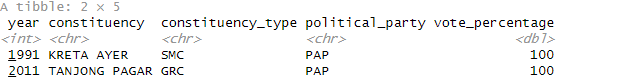
1
2
3
4
df.ge.results %>%
  filter((year == 1991 & constituency_type == "SMC" & vote_percentage == 100) |
         (year == 2011 & constituency_type == "GRC" & vote_percentage == 100)) %>%
  select(year, constituency, constituency_type, political_party, vote_percentage)
Figure 6b
1
2
3
df.ge.results %>%
  filter(constituency == "HOUGANG" & year >= 1988) %>%
  select(year, constituency, political_party)
Figure 7
Another important component of Singapore’s parliamentary election is the call for by-elections, which may give parties a chance to flip seats in their favor while extending their influence in parliament. The path plot is used to portray such changes. In terms of data pre-processing, a new data frame ‘df.combined.filter’ is created, taking reference from ‘df.combined.results’ where filter() is applied to sieve out observations from “elected” variable that are neither “NA” nor empty. An extract of the code is reproduced below for reference:
1
2
3
4
5
6
7
8
9
10
11
12
13
14
15
16
17
18
19
20
21
22
23

# Create data frame while filtering out blank observations
df.combined.filter <- df.combined.results %>%
  filter(!is.na(elected) & elected != "")

# Create path plot
ggplot(df.combined.filter, aes(x = year, y = constituency, color = party_category, group = constituency)) +
  geom_path(size = 1) +
  geom_point(size = 3) +
  scale_color_manual(values = c("WP" = "dodgerblue3", "PAP" = "maroon2", "Other Opposition" = "coral3")) +
  labs(title = "Figure 7 : Flipping of Constituencies Over Time",
       subtitle = "PAP possesses a strong track record in flipping constituencies in their favour",
       caption = "Source: Data.gov.sg",
       x = "Year",
       y = "",
       color = "Political Party") +
  theme_minimal() +
  theme(
    axis.title.y = element_blank(),
    plot.title = element_text(size = 20, face = "bold"),
    plot.subtitle = element_text(size = 16),
    axis.title.x = element_text(size = 14),
    axis.text = element_text(size = 12, face = "bold"))
Figure 8a and 8b
The leaflet and waffle plots are used to represent seats won by geographical area and visualise changes to parliamentary seat composition respectively. In terms of data pre-processing, a new data frame ‘df.ge.results.20XX’ is created by filtering the year to its respective election period and where seat variable is not 0 referenced from ‘df.ge.results’. Next, the ‘left_join()’ function is used to append all variables from ‘df.ge.results.20XX’ with “constituency” as the primary key for left join. As there are by-elections conducted for 2011 and 2015 elections, specific rows are extracted from ‘df.be.results’ before appending them into ‘df.ge.results.20XX’. The original election results for that constituency is superseded by the by-election results, thus removal of specific rows are performed to achieve the updated results. An extract of the code is reproduced below for reference:
1
2
3
4
5
6
7
8
9
10
11
12
13
14
15
16
17
18
19
20
21
22
23
24
25
26
27
28
29
30
31
32
33
34
35
36
37
38
39
40
41
42
43
44
45
46
47
48
49
50
51
52
53
54
55
56
57
58

# Install phantomjs and to load leaflet and htmlwidget libraries
webshot::install_phantomjs(force = TRUE)
library(htmlwidgets)
library(leaflet)

# Create new data frame by filtering variables in 'df.ge.results' for plotting
df.ge.results.2006 <- df.ge.results %>%
  filter(year == 2006 & seats != 0) %>%
  select(constituency, constituency_type, seats, elected)

# Left Join 'df.boundaries.2006' and 'df.ge.results.2006'
gemap.2006 <- left_join(df.boundaries.2006, df.ge.results.2006, by = "constituency")

# Set party colors
party_colors <- colorFactor(
  palette = c("PAP" = "snow2", "SDA" = "orange", "WP" = "dodgerblue3"),
  domain = gemap.2006$elected)

# Create leaflet plot
leaflet_map_2006 <- leaflet(data = gemap.2006) %>%
  addProviderTiles(providers$OpenStreetMap) %>%
  addPolygons(
    fillColor = ~party_colors(elected),
    label = ~paste(constituency, constituency_type, ",", elected, ":", seats, "Seat(s) Won"),
    color = "black",
    weight = 1,
    opacity = 1,
    fillOpacity = 0.7) %>%
  addLegend(
    position = "bottomright",
    title = "Singapore Parliamentary Elections 2006",
    pal = party_colors,
    values = ~elected)

# Save the Leaflet map as an HTML file
saveWidget(leaflet_map_2006, "leaflet_map_2006.html")

# Take a screenshot of HTML file and save it as a png file
webshot::webshot("leaflet_map_2006.html", "leaflet_map_2006.png")

# Load waffle library
library(waffle)

## Creating waffle plot

# Create data frame summing seats
seats.2006 <- df.ge.results.2006 %>%
  group_by(elected) %>%
  summarise(total_seats = sum(seats)) %>%
  deframe()

# Create the waffle plot
waffle(seats.2006, rows = 7, colors = c("snow2", "orange", "dodgerblue3")) +
  labs(title = "Seats Won by Each Party in 2006",
       subtitle = "The rise of opposition parties") +
  theme(plot.title = element_text(size = 20, face = "bold"),
        plot.subtitle = element_text(size = 18))
Figure 9a and 9b
1
2
3
4
5
6
7
8
9
10
11
12
13
14
15
16
17
18
19
20
21
22
23
24
25
26
27
28
29
30
31
32
33
34
35
36
37
38
39
40
41
42
43
44
45
46
47
48
49
50
51
52
53
54
55
56

# Create new data frame by filtering variables in 'df.ge.results' for plotting
df.ge.results.2011 <- df.ge.results %>%
  filter(year == 2011 & seats != 0) %>%
  select(constituency, constituency_type, seats, elected)

# Select the specific rows from 'df.be.results'
selected.rows.2011 <- df.be.results[c(64,67), ] %>%
  select(constituency, constituency_type, seats, elected)

# Append by-election data within 'df.ge.results.2011'
df.ge.results.2011 <- bind_rows(df.ge.results.2011, selected.rows.2011)

# Remove rows superseded by constituencies where by-election was held
df.ge.results.2011 <- df.ge.results.2011 %>%
  slice(-c(9, 19))

# Left Join 'df.boundaries.2011' and 'df.ge.results.2011'
gemap.2011 <- left_join(df.boundaries.2011, df.ge.results.2011, by = "constituency")

# Create leaflet plot
leaflet_map_2011 <- leaflet(data = gemap.2011) %>%
  addProviderTiles(providers$OpenStreetMap) %>%
  addPolygons(
    fillColor = ~party_colors(elected),
    label = ~paste(constituency, constituency_type, ",", elected, ":", seats, "Seat(s) Won"),
    color = "black",
    weight = 1,
    opacity = 1,
    fillOpacity = 0.7) %>%
  addLegend(
    position = "bottomright",
    title = "Singapore Parliamentary Elections 2011 (adjusted for by-election)",
    pal = party_colors,
    values = ~elected)

# Save the Leaflet map as an HTML file
saveWidget(leaflet_map_2011, "leaflet_map_2011.html")

# Take a screenshot of HTML file and save it as a png file
webshot::webshot("leaflet_map_2011.html", "leaflet_map_2011.png")

## Creating waffle plot

# Create data frame summing seats
seats.2011 <- df.ge.results.2011 %>%
  group_by(elected) %>%
  summarise(total_seats = sum(seats)) %>%
  deframe()

# Create the waffle plot
waffle(seats.2011, rows = 7, colors = c("snow2", "dodgerblue3")) +
  labs(title = "Seats Won by Each Party in 2011 (adjusted for by-election)",
       subtitle = "A historical milestone for WP") +
  theme(plot.title = element_text(size = 20, face = "bold"),
        plot.subtitle = element_text(size = 18))
Figure 10a and 10b
1
2
3
4
5
6
7
8
9
10
11
12
13
14
15
16
17
18
19
20
21
22
23
24
25
26
27
28
29
30
31
32
33
34
35
36
37
38
39
40
41
42
43
44
45
46
47
48
49
50
51
52
53
54
55
56

# Create new data frame by filtering variables in 'df.ge.results' for plotting
df.ge.results.2015 <- df.ge.results %>%
  filter(year == 2015 & seats != 0) %>%
  select(constituency, constituency_type, seats, elected)

# Select the specific rows from 'df.be.results'
selected.rows.2015 <- df.be.results[70, ] %>%
  select(constituency, constituency_type, seats, elected)

# Append by-election data within 'df.ge.results.2015'
df.ge.results.2015 <- bind_rows(df.ge.results.2015, selected.rows.2015)

# Remove rows superseded by constituencies where by-election was held
df.ge.results.2015 <- df.ge.results.2015 %>%
  slice(-4)

# Left Join 'df.boundaries.2015' and 'df.ge.results.2015'
gemap.2015 <- left_join(df.boundaries.2015, df.ge.results.2015, by = "constituency")

# Create leaflet plot
leaflet_map_2015 <- leaflet(data = gemap.2015) %>%
  addProviderTiles(providers$OpenStreetMap) %>%
  addPolygons(
    fillColor = ~party_colors(elected),
    label = ~paste(constituency, constituency_type, ",", elected, ":", seats, "Seat(s) Won"),
    color = "black",
    weight = 1,
    opacity = 1,
    fillOpacity = 0.7) %>%
  addLegend(
    position = "bottomright",
    title = "Singapore Parliamentary Elections 2015 (adjusted for by-election)",
    pal = party_colors,
    values = ~elected)

# Save the Leaflet map as an HTML file
saveWidget(leaflet_map_2015, "leaflet_map_2015.html")

# Take a screenshot of HTML file and save it as a png file
webshot::webshot("leaflet_map_2015.html", "leaflet_map_2015.png")

## Creating waffle plot

# Create data frame summing seats
seats.2015 <- df.ge.results.2015 %>%
  group_by(elected) %>%
  summarise(total_seats = sum(seats)) %>%
  deframe()

# Create the waffle plot
waffle(seats.2015, rows = 7, colors = c("snow2", "dodgerblue3")) +
  labs(title = "Seats Won by Each Party in 2015 (adjusted for by-election)",
       subtitle = "PAP retained Bukit Batok SMC and flipped Punggol East SMC but WP held firm") +
  theme(plot.title = element_text(size = 20, face = "bold"),
        plot.subtitle = element_text(size = 18))
Figure 11a and 11b
1
2
3
4
5
6
7
8
9
10
11
12
13
14
15
16
17
18
19
20
21
22
23
24
25
26
27
28
29
30
31
32
33
34
35
36
37
38
39
40
41
42
43
44
45

# Create new data frame by filtering variables in 'df.ge.results' for plotting
df.ge.results.2020 <- df.ge.results %>%
  filter(year == 2020 & seats != 0) %>%
  select(constituency, constituency_type, seats, elected)

# Left Join 'df.boundaries.2020' and 'df.ge.results.2020'
gemap.2020 <- left_join(df.boundaries.2020, df.ge.results.2020, by = "constituency")

# Create leaflet plot
leaflet_map_2020 <- leaflet(data = gemap.2020) %>%
  addProviderTiles(providers$OpenStreetMap) %>%
  addPolygons(
    fillColor = ~party_colors(elected),
    label = ~paste(constituency, constituency_type, ",", elected, ":", seats, "Seat(s) Won"),
    color = "black",
    weight = 1,
    opacity = 1,
    fillOpacity = 0.7) %>%
  addLegend(
    position = "bottomright",
    title = "Singapore Parliamentary Elections 2020",
    pal = party_colors,
    values = ~elected)

# Save the Leaflet map as an HTML file
saveWidget(leaflet_map_2020, "leaflet_map_2020.html")

# Take a screenshot of HTML file and save it as a png file
webshot::webshot("leaflet_map_2020.html", "leaflet_map_2020.png")

## Creating waffle plot

# Create data frame summing seats
seats.2020 <- df.ge.results.2020 %>%
  group_by(elected) %>%
  summarise(total_seats = sum(seats)) %>%
  deframe()

# Create the waffle plot
waffle(seats.2020, rows = 7, colors = c("snow2", "dodgerblue3")) +
  labs(title = "Seats Won by Each Party in 2020",
       subtitle = "WP achieved yet another historical milestone by securing 2 GRCs and 10 seats") +
  theme(plot.title = element_text(size = 20, face = "bold"),
        plot.subtitle = element_text(size = 18))
Figure 12
Recently, Singapore’s political landscape have been heavily impacted by scandals and negative limelight, leading to the highest number of resignations by MPs since the political boycott in 1968. WP vacated 2 seats and the PAP vacated 4 seats ahead of the 2025 parliamentary election. Adjustments were made to deduct vacated seats from each party before visualising them via a waffle plot. An extract of the code is reproduced below for reference:
1
2
3
4
5
6
7
8
9
10
11
12
13
14
15
16
17
18
19
20

## Creating waffle plot

# Create data frame summing seats
seats.2024 <- df.ge.results.2020 %>%
  group_by(elected) %>%
  summarise(total_seats = sum(seats)) %>%
  deframe()

# Adjust seat counts for WP and PAP and add "Vacated" category
seats.2024["WP"] <- seats.2024["WP"] - 2
seats.2024["PAP"] <- seats.2024["PAP"] - 4
seats.2024["Vacated"] <- 6

# Create the waffle plot
waffle(seats.2024, rows = 7, colors = c("snow2", "dodgerblue3", "springgreen2")) +
  labs(title = "6 Vacated Seats in Parliament",
       subtitle = "Fielding strong replacements required for both PAP and WP to fill 6 vacated seats") +
  theme(plot.title = element_text(size = 20, face = "bold"),
        plot.subtitle = element_text(size = 18))
Figure 13
1
2
3
df.ge.results %>%
  filter(elected == "PAP" & year == 2020 & margin_gap < 10) %>%
  select(year, constituency, constituency_type, political_party, margin_gap, seats)
Figure 14
1
2
3
df.ge.results %>%
  filter(elected == "WP" & year == 2020 & margin_gap < 10) %>%
  select(year, constituency, constituency_type, political_party, margin_gap, seats)